Sorting Algorithms Overview: Theory and Visualization

Sorting algorithms are a staple of programming proficiency: whatever your stack is, great knowledge of algorithms really sets you apart from your competitors. It’s easy to see why — languages and frameworks come and go, but foundational computer science knowledge (which is almost synonymous with proficiency in algorithms) is always in demand. One good way of staying at the top of your game is listening to podcasts — their creators will cover all the topics you’re interested in.

Once a web developer has learned modern front- or back-end technologies, they need to master sorting algorithms to really let their expertise shine — so in this article, we’ve prepared a compendium of the most popular sorting algorithms coupled with both theoretical and practical questions which can really test your knowledge.

Theory

As sorting algorithms feature a lot of theoretical knowledge, we can try and assess just how well you know the most popular ones: bubble sort, quick sort, merge sort, selection sort, and heap sort. How are they structured? What are their pros and cons? Where can they be used optimally? Let’s find out! And stay tuned for the article which will cover practical algorithms-related interview questions – we’ll publish it soon. 🙂

Bubble sort

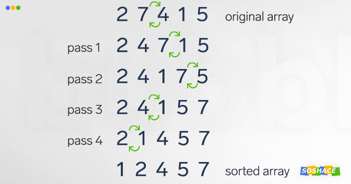How does it work? With each pass, the algorithm divides the adjacent array items in pairs and scans them, swapping the items in a pair when a given pair is in the wrong order. Each pass leads to the next largest item being pushed to the end of the array, similar to how bubbles are pushed to the top of a drink (this is where this algorithm takes its name from). The passes are then repeated until the array is finally sorted and no swaps are required, indicating that the element order is correct.

def bubbleSort(arr):
    n = len(arr)

    # Traverse through all array elements
    for i in range(n):
        swapped = False

        # Last i elements are already
        #  in place
        for j in range(0, n - i - 1):

            # traverse the array from 0 to
            # n-i-1. Swap if the element
            # found is greater than the
            # next element
            if arr[j] > arr[j + 1]:
                arr[j], arr[j + 1] = arr[j + 1], arr[j]
                swapped = True

        # IF no two elements were swapped
        # by inner loop, then break
        if swapped == False:
            break

# Driver code to test above


arr = [64, 34, 25, 12, 22, 11, 90]

bubbleSort(arr)

print("Sorted array :")
for i in range(len(arr)):
    print("%d" % arr[i], end=" ")

What are its drawbacks/limitations? Bubble sort is the most basic of the algorithms we’ll be reviewing in this article — and it’s also the easiest to criticize: even though simplicity is often appreciated in programming, the oversimplicity of bubble sort presents a number of limitations. Despite the fact that it’s quite stable and easy to understand,

How can it be optimized? Although bubble sort algorithm is generally considered to be rather inefficient, it still might be useful in some situations: for instance, a sorted array has one element that gets incremented — then one walk through the array will sort it in an efficient manner.

Selection sort

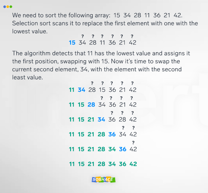How does it work? A counterpart of bubble sort, selection sort is another in-place comparison sort, In addition, it has the upper hand over more intricate algorithms in situations where auxiliary memory is concerned — and in small arrays as well. Here’s how it works:

1. The array is divided into subarrays — sorted and unsorted.
2. It recursively looks for the minimum element (in the unsorted subarray) and puts it at the beginning (in the sorted one)

# code courtesy of George Seif @george.seif94
def selection_sort(arr):
    for i in range(len(arr)):
        minimum = i

        for j in range(i + 1, len(arr)):
            # Select the smallest value
            if arr[j] < arr[minimum]:
                minimum = j

        # Place it at the front of the
        # sorted end of the array
        arr[minimum], arr[i] = arr[i], arr[minimum]

    return arr

What are its drawbacks/limitations? Due to its O(n²) time complexity, it performs inefficiently in large arrays (coupled with the fact that it’s generally outperformed by its counterpart, insertion sort). Compared to insertion sort, this algorithm has to scan each remaining element to proceed, while insertion sort only scans as many elements as needed — this means that selection sort normally performs twice as many operations. Furthermore, in-place comparison algorithms like a bubble, selection, and insertion sort are suboptimal for large arrays where divide-and-conquer algorithms reign supreme.

How can it be optimized? Curiously enough, a whole study has been dedicated to creating an optimized version of selection sort, called optimized selection sort — it claims that the optimized version is 2x faster, and performs less data exchange.

Insertion sort

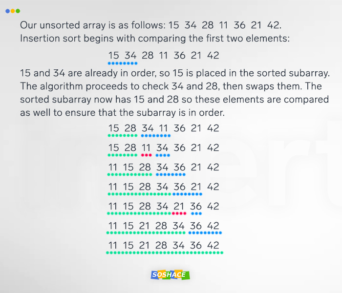How does it work? Out of all in-place comparison algorithms, insertion sort offers both the best performance and, arguably, the best design. It excels in small arrays and nearly-sorted data, almost reaching O(n) complexity. Additionally, it doesn’t require auxiliary storage thanks to its in-place nature. Here’s how it’s structured: The array is divided into two subarrays — sorted and unsorted. The algorithm performs sequential scans, checking whether element pairs are in order and sending elements that meet this criterion in the sorted subarray.

# code courtesy of George Seif @george.seif94
def insertion_sort(arr, simulation=False):

    for i in range(len(arr)):
        cursor = arr[i]
        pos = i

        while pos > 0 and arr[pos - 1] > cursor:
            # Swap the number down the list
            arr[pos] = arr[pos - 1]
            pos = pos - 1
        # Break and do the final swap
        arr[pos] = cursor

    return arr

What are its drawbacks/limitations? Like all in-place comparison algorithms, it performs poorly in large data sets. Speaking of large data sets: we have a list of SQL interview questions!

How can it be optimized? Just like in selection sort’s case, there are studies which explore how it can be optimized. To address the problems of large arrays (where this type of algorithm performs poorly), we can utilize the hybrid approach: once the array has been scaled down to a smaller size, in-place comparison algorithms comes into play.

Quick sort

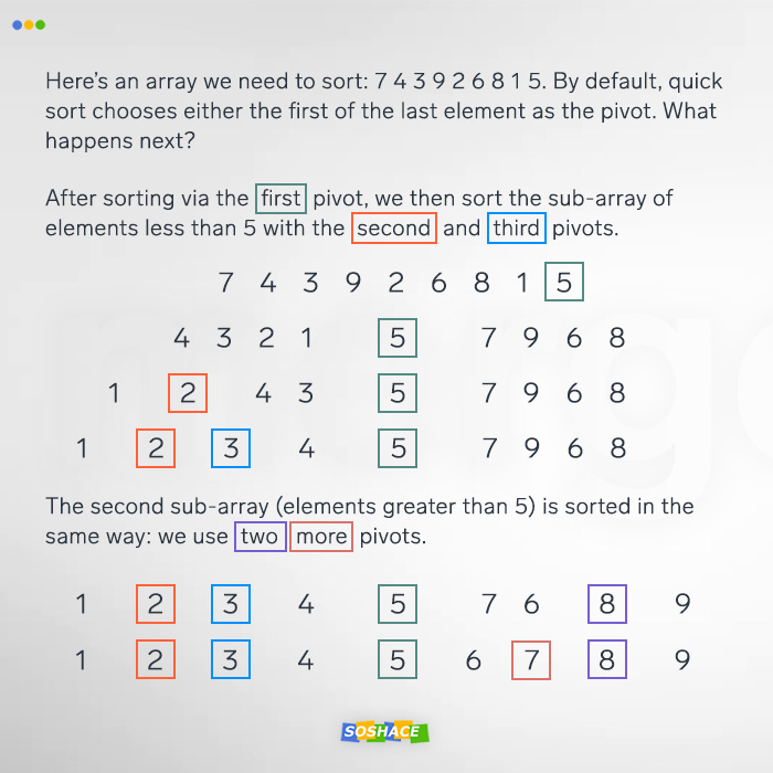How does it work? In most situations, quick sort is the fastest and most efficient algorithm, easily outperforming merge sort and heapsort. Since it operates via comparisons, it requires less-than relation definitions of the array elements. Following the divide and conquer pattern, it starts off with separating the large array into smaller arrays, then sorts the smaller ones recursively. In essence, the algorithm follows this structure:

1. Choosing pivot, an element from the array which other elements will be compared against.
2. Partitioning, i.e. moving the elements with values less than that of the pivot to the left; moving the elements with values greater than that of the pivot to the right.
3. Re-applying steps 1 and 2 to the newly-formed subarrays.

# code courtesy of George Seif @george.seif94
def partition(array, begin, end):
    pivot_idx = begin
    for i in xrange(begin + 1, end + 1):
        if array[i] <= array[begin]:
            pivot_idx += 1
            array[i], array[pivot_idx] = array[pivot_idx], array[i]
    array[pivot_idx], array[begin] = array[begin], array[pivot_idx]
    return pivot_idx


def quick_sort_recursion(array, begin, end):
    if begin >= end:
        return
    pivot_idx = partition(array, begin, end)
    quick_sort_recursion(array, begin, pivot_idx - 1)
    quick_sort_recursion(array, pivot_idx + 1, end)


def quick_sort(array, begin=0, end=None):
    if end is None:
        end = len(array) - 1

    return quick_sort_recursion(array, begin, end)

What are its drawbacks/limitations? When an input contains a large number of repeating/equal items, the algorithm’s performance decreases significantly. Furthermore, choosing either the smallest or the largest element of the array as the pivot leads to the worst-case time complexity.

How can it be optimized? There are a few techniques we can use to make quick sorting more efficient:

• Choosing the right pivot — the element which the list will be partitioned around. As showcased above, the pivot can make or break this algorithm; by default, either the leftmost or rightmost element of the partition is chosen as the pivot — and this leads to the worst performance. To solve this problem, we have two options: 1) choosing a random index for the pivot or 2) choosing the median of three elements (most often the first, middle, and last.
• To handle repeated elements (e.g. when all input elements are equal) more efficiently, we can make the algorithm group the elements into 3 subarrays: 1) less-than-pivot; 2) equal-to-pivot; 3) more-than-pivot.
• Using Hoare’s partition scheme: two indices (the leftmost and the rightmost elements) move toward each other until they find a pair of elements (one less than the pivot, one greater) which are out of order. These elements are then swapped.

Merge sort

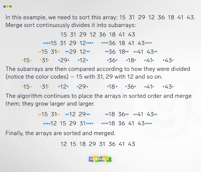How does it work? This algorithm shares many similarities with quick sort: it boasts efficiency coupled with comparison-based nature and “divide and conquer” pattern. The steps that it follows are:

1. Repeatedly group the array into a number of subarrays until each subarray only contains a single element. Divide the unsorted list into n sublists, each containing one element (a list of one element is considered sorted).
2. Recursively merge subarrays, creating new sorted subarrays until only one remains — this last one will be sorted.

# code courtesy of George Seif @george.seif94
def merge_sort(arr):
    # The last array split
    if len(arr) <= 1:
        return arr
    mid = len(arr) // 2
    # Perform merge_sort recursively on both halves
    left, right = merge_sort(arr[:mid]), merge_sort(arr[mid:])

    # Merge each side together
    return merge(left, right, arr.copy())


def merge(left, right, merged):

    left_cursor, right_cursor = 0, 0
    while left_cursor < len(left) and right_cursor < len(right):

        # Sort each one and place into the result
        if left[left_cursor] <= right[right_cursor]:
            merged[left_cursor + right_cursor] = left[left_cursor]
            left_cursor += 1
        else:
            merged[left_cursor + right_cursor] = right[right_cursor]
            right_cursor += 1

    for left_cursor in range(left_cursor, len(left)):
        merged[left_cursor + right_cursor] = left[left_cursor]

    for right_cursor in range(right_cursor, len(right)):
        merged[left_cursor + right_cursor] = right[right_cursor]

    return merged

What are its drawbacks/limitations? As merge- and quicksort share a lot of similarities, comparing them directly allows us to see a number of problems of merge sort:

• Additional space: unlike quick sort, merge sort needs a temporary array which it uses to merge its subarrays.
• Locality of reference: merge sort handles cache locality far worse.
• Suboptimal for small data structures.

How can it be optimized? One method of optimization is to reduce the number of instances when pages enter and leave the computer’s memory cache — the tiled merge sort utilizes this principle. Another is to perform each pass in lock-step, without creating unnecessary copies in the merge-sort tree.

Conclusion

For many developers, sorting algorithms are shrouded in mystery: they often seem too math-heavy or too computer science-y. In reality, however, every web developer (remote or in-office) always works with data — and knowing how to sort this data well is yet another stepping stone to becoming even better. (That’s what our blog is aimed at — helping you improve your web development skills even further 🙂 )